


Attention is Transformer’s breath,
Multi-Head is Transformer’s release,
RNNs thou wert and art,
May thy model reach to greater accuracy.
Látom.
- Enen No Shouboutai
I'm getting tired of butchering anime and video game quotes so I'm thinking I should butcher some meme quotes next time. Anyways, well I have been writing on a lot of topics but something I always wanted to write about is probably explaining a research paper.
I mean I've been seeing blogs that go by the name of Paper Dissected so I wanted to try writing one myself. Well this is going to be my first try in this and frankly, I have no idea how it'll be but let's give it a try, shall we?
I guess it's safe to say that Attention Mechanism and Transformers is something that recently took over NLP. Not only did it show improvements over the SOTA models at the time but also overcome the shortcoming of the RNN models like LSTM and GRU.
So let's go ahead and break down the sections of the paper, Attention is all you need. To give you a gist of what'll be there, it'll be an explanation of each section in the paper like abstract, introduction, model architecture, etc.
Abstract
This section pretty much summarizes the whole paper not in terms of working but rather in terms of what it has to offer. It starts with explaining how Seq2Seq models usually use RNN and CNN for encoder and decoder, and how the best ones connect encoder and decoder via attention mechanism.
Now just to be clear, attention itself is not a new concept but to rely completely on attention is something that this paper introduced. It went ahead explaining the results achieved on the machine translation task which were like the following on WMT-2014 dataset:-
| MT - Task | BLEU Score |
| English to German | 28.4 |
| English to French | 41.8 |
It also took 3.5 days and 8 GPUs to train on, which is certainly out of my budget. But the main thing that shined a bit differently than others in the abstract section was:-
Experiments on two machine translation tasks show these models to be superior in quality while being more parallelizable and requiring significantly less time to train.
We saw how results were better than traditional models but the thing that separated transformers from LSTM is parallel computation. This can feel a bit tricky to understand at the start so let's break it down. By nature, RNN models aren't parallel but rather Sequential and this is because they compute results one step at a time.
However, in the Transformer model, there is no such thing as "time steps" but rather the inputs are passed all together and all this is made possible due to multi-headed attention and other stuff which we'll talk about later.
Introduction
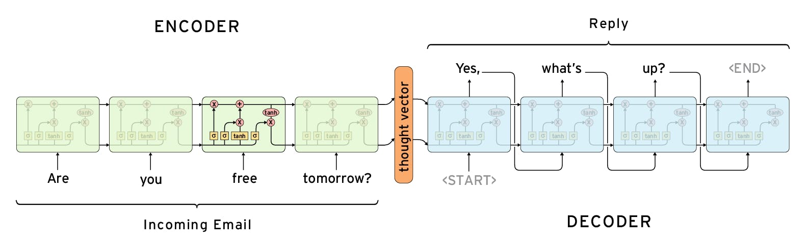
This section mainly talks about the working of RNNs and it's limitations, along with the recent developments to tackle them. Now that we are at it let's understand how does Seq2Seq modeling working in the case of RNNs and to make it easier, take a look a look at the picture below:-
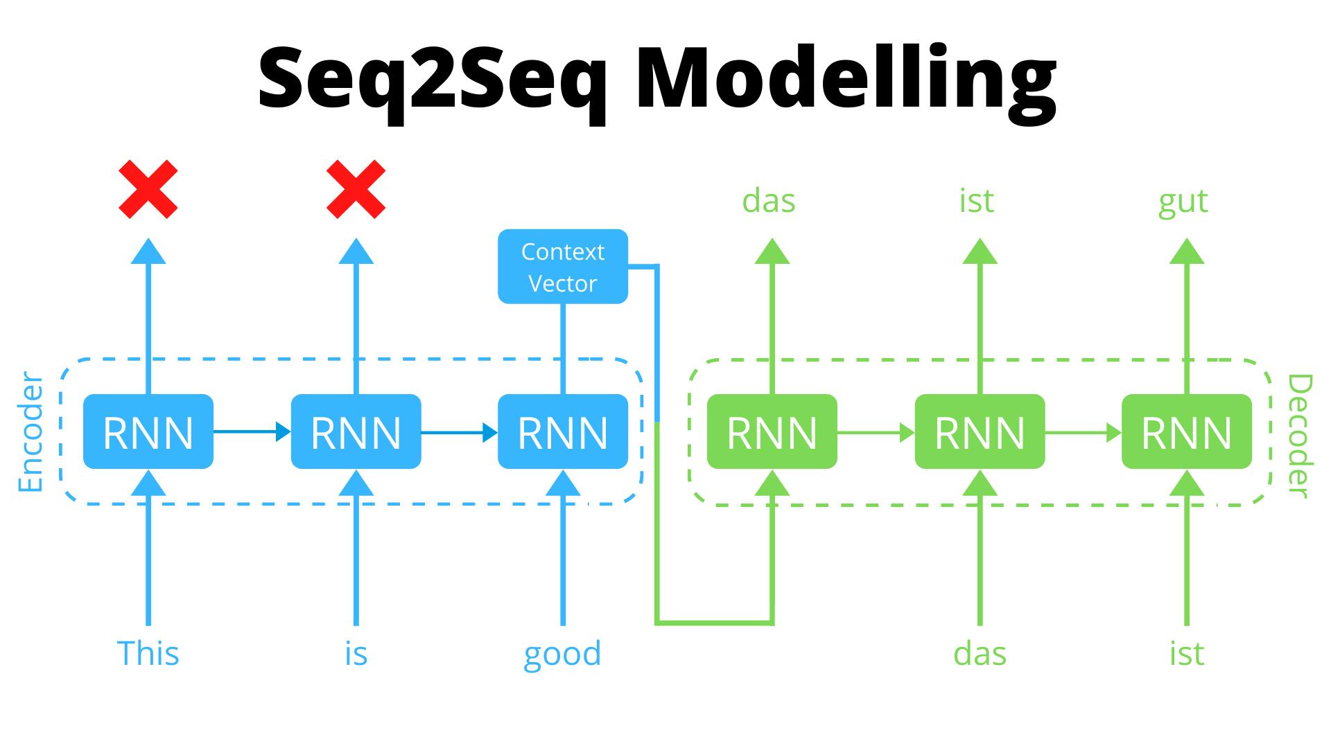
Seq2Seq Models consists of 2 models i.e. an Encoder and a Decoder. The Encoder model takes the text as input and generates a Context Vector as an output which is nothing but the last hidden state of RNN. Encoders and Decoders are nothing but RNNs and in few instances CNN 🌚.
Another thing you'll notice is the crosses above RNN cells except the last one that doesn't mean they aren't produced, they are but we just don't use them and all we'll be doing is to take the context vector from the last time step and feeding it to the decoder as input who'll output each word at a time giving us the resultant text.
In attention, however, you'll be taking the outputs of all the time step of encoder so you don't discard in that case. I mean you can also do mean pooling on all the states and pass that as context vector, so attention isn't the only way that uses all the states. But how does the decoder predict the words? Let's see, I'll try to be brief.
In the decoder, the first token is the special token signifying the start of the sentence along with the context vector from the encoder, after that you pass the previous output as input to the decoder along with the hidden state to generate new output. However during training, we feed the ground-truth value of targets as input to the decoder, this is known as Teacher Forcing. Without which the model weights will be updated on inferred text making it difficult for model to learn from.
However during inference, you'll use generated output as input to generate the next token, and it's cool except the output is being constructed on the context of inferred output rather than actual ones, which causes discrepancy during training and inference, giving rise to the problem of exposure bias.
Back to the topic, the nature of RNNs is sequential which makes parallelization difficult for training, making RNN models take more time to train. However, there are few developments that tackle it:-
Recent work has achieved significant improvements in computational efficiency through factorization tricks and conditional computation, while also improving model performance in the case of the latter. The fundamental constraint of sequential computation, however, remains.
To understand the factorization trick you can go ahead and read another paper, i.e. Factorization Tricks for LSTM Networks by Oleksii and Boris, which I recommend but I'll give you the gist of it.
The major part of LSTMP cell computation is in computing affine transform T because it involves multiplication with 4n × 2p matrix W.
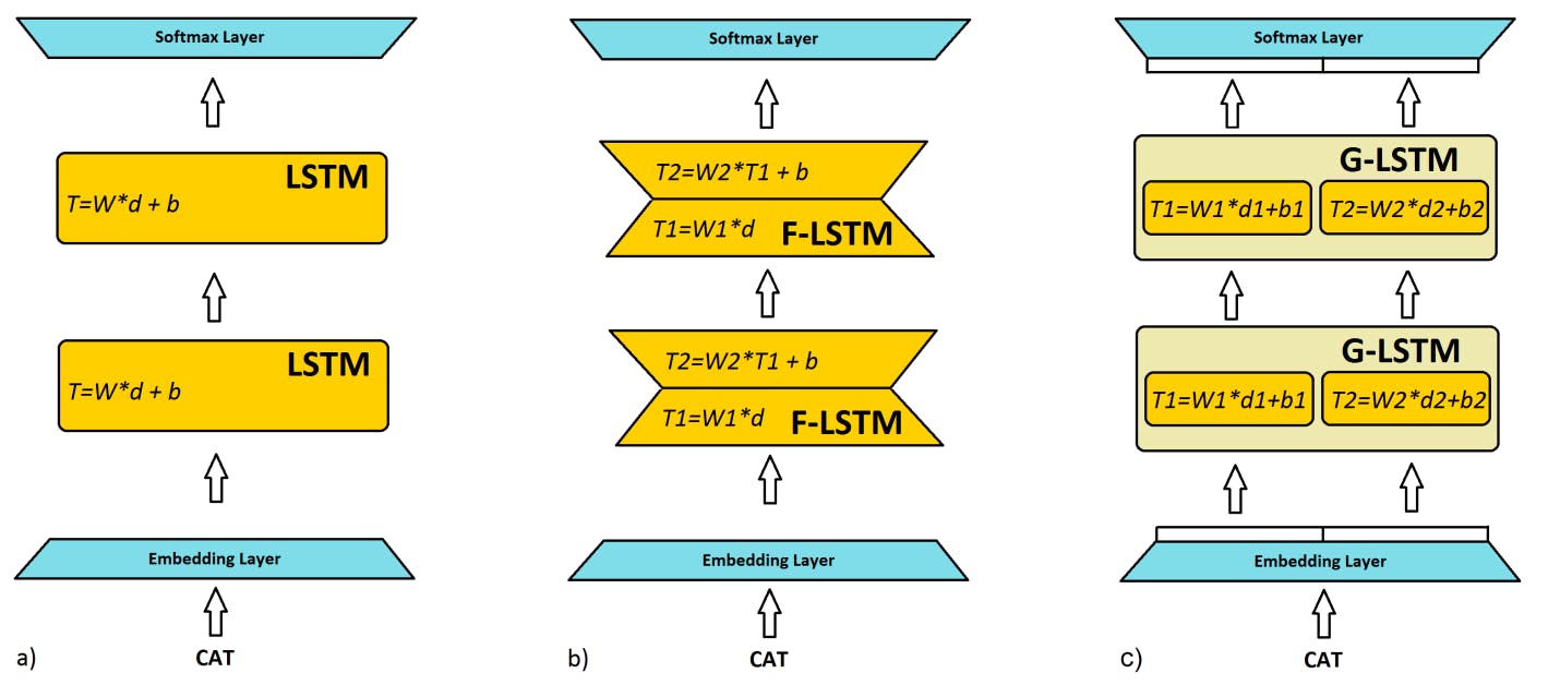
The aim of the factorization trick is to approximate that W by replacing it with the product of 2 matrices W1(2p*r) and W2(r*4n), this way takes fewer parameters (2pr + r4n) as compared to W (2p*4n) given r < p <=n. Another factorization trick proposes to think parts of inputs and the hidden states as independent of each other and calculate affine transforms of these groups individually and parallelly.
I know it's a lot to grasp so if you don't understand it all at the moment it's fine, important thing to understand is that many attempts have been made to improve RNNs but the sequential nature isn't completely removed. The attention model did help in capturing long-term dependencies and improve results, however, it was used along with RNNs.
There is another concept of conditional computation that aims at activating parts of the network to improve computational efficiency, and performance too in this case, but let's not dive much into it. But if you want to you can read this short book on the same.
The transformer model on the other hand relies entirely on attention mechanism allowing it to be more parallelizable and give better results with the cost of training being 12 hours on 8 P100 GPUs, something that even Colab Pro users can't get their hands on all the time anymore 🥲.
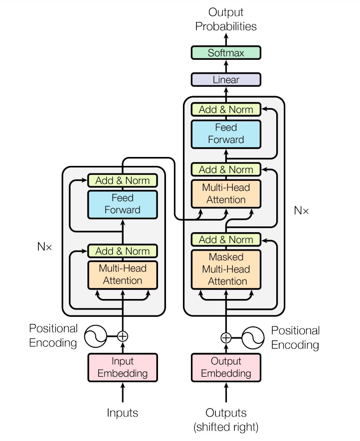
Model Architecture
Finally, we've come to the real deal. Now while I wanna try and break down the explanation sub-section wise, I know that may or may not end up leaving you kinda confused, and hence instead of explaining each sub-section of this section we'll dismantle the architecture step by step and understand how it works.
Input Embeddings
Let's start from the beginning, what you have with you is a sentence or bunch of sentences. Now you can't exactly feed it to the model as it is so you need a way to convert it to a form more suitable for it. When we used RNNs for text classification or seq2seq we convert our text to word embeddings.
These embeddings are nothing but vector representations of words such that words with similar meanings are closer to each other. But what does closer mean? Mathematically, closer means the similarity score is high. This score can be anything but cosine similarity is popular so feel free to think that. Once we have our embeddings to use we are all set! Are we?

Technically, yes we are since these embeddings can be used with RNNs and CNNs because they are able to capture the ordering into consideration. But Transformers use only self-attention, which takes all the words at the same time hence it is not able to take the order of words into consideration. To fix this problem we introduce something called positional encodings.
Positional Encodings
So as mentioned before, inherently attention model is not able to take the order of words into consideration. In order to compensate for this, we use something called Positional Encodings. Don't be intimidated by the name it's actually much more simple. Let's dive a bit deeper into this.
Need of Positional Encodings
When working with text it's really important to take words order into consideration. Why? The order of words defines the structure of the sentence and this structure helps in providing the context.
RNNs by nature are sequential in nature by taking inputs one by one and updating hidden states accordingly, but the same is not the case with attention since it takes the words all at once. Why this is so, is something we'll understand in the next section but for now, let's say that's how it is.
So we need some extra sources of information in our embeddings to convey this information, something that could tell the position of a word in a sentence. To do so we can add an extra embedding or matrix to our word embeddings to provide info regarding the ordering of the word. But how?
Finding Positional Encodings
Well in the most simple case you can use a one-hot encoded form of [0,1,2,3,4,5,..., pos] as positional encodings. You can train an embedding layer to find the positional embedding matrix, where each row has the positional embedding for word at pos index, for this and add it to input embeddings.
In the paper, however, the proposed approach uses a combination of sin and cos function to find the encodings. Take a look at the following picture:-
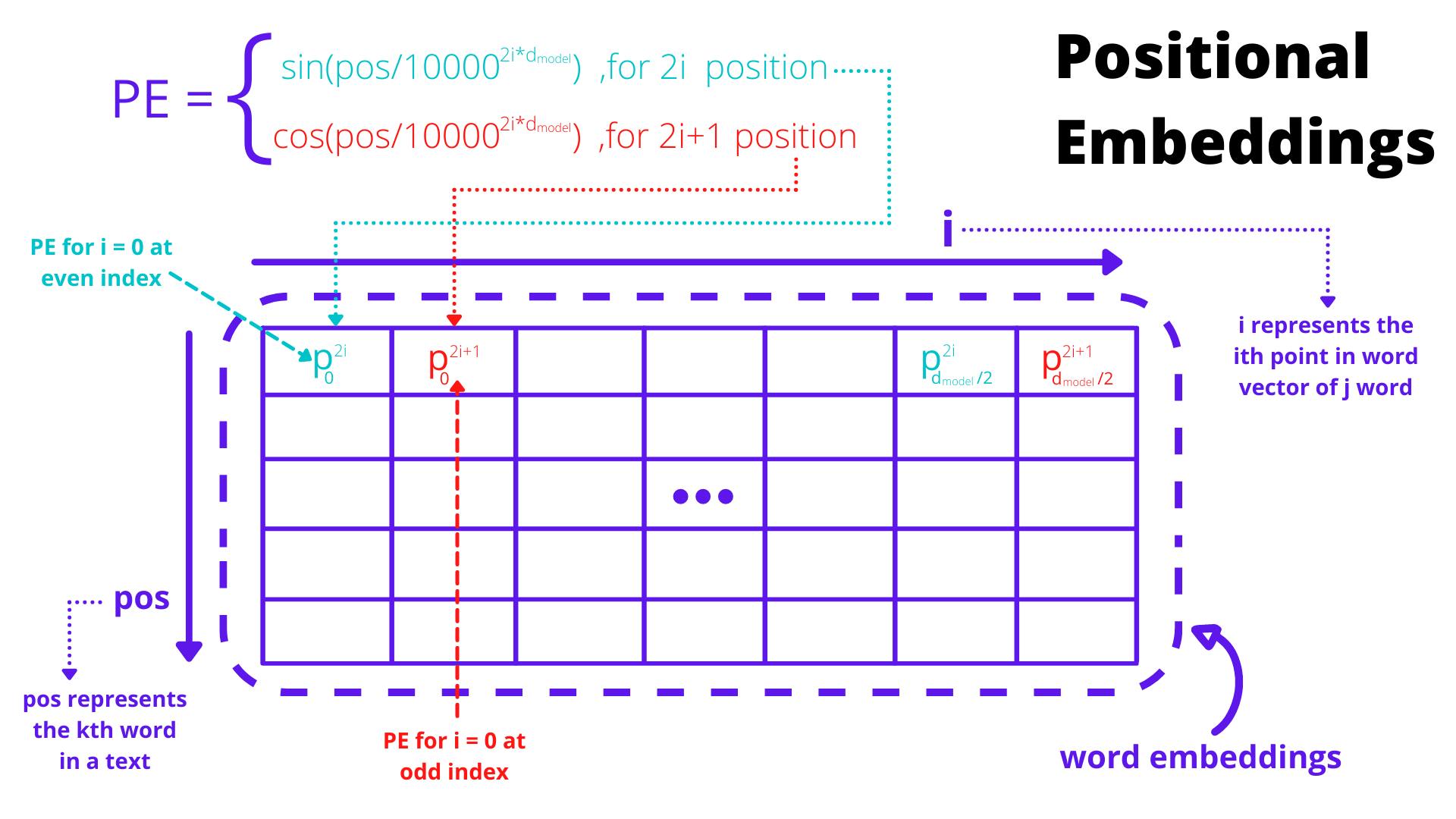
As you can see in the above picture the encodings are found by using a combination of sin and cos function. The function is quite self-explanatory, it says that for the embedding of a word at position pos:-
The value at index 2i is given using the sin function, colored red.
The value at index 2i +1 is given using the cos function, colored blue.
But why are we using this particular function? Well let's hear from the authors themselves:-
We chose this function because we hypothesized it would allow the model to easily learn to attend by relative positions since, for any fixed offset k, PEpos+k can be represented as a linear function of PEpos.
Well, researchers sure love to make stuff seem more complicated, don't they? It's fine if you don't understand the above sentence, take it as a confirmation that you're still sane.
What the sentence means to say is that given the positional encoding of the word at pos you can find the positional encoding of word at pos + k by applying some linear transformation on the positional encoding of pos. Mathematically, it can be written like this:-
\[PE_{p+k} = T * PE_p\]
Writing pos as p in the above equation since latex is getting messed up for some reason. The important thing to know is that the matrix T can be used to find PE at pos+k but what is this T? Can we find it? Well yes, that T is a rotational matrix that depends on offset k rather than pos. Wait what! How?
Well, you can derive it, and here is a really good blog by Amirhossein doing the same. There is another blog by Timo Denk that proves the linear relationship between PE at pos and pos+k but the first one explains in a much simpler fashion, but do give both a read.
Improving a bit more
Wow so everything is dope, right? Fortunately or unfortunately, No. Even though everything might seem super nice with these encodings, which it is, what these really are doing is finding values for given pos and i values, these are also called Absolute Positional Encodings. While the altering of sin and cosine might be able to add relative nature, we might actually have something better i.e. Relative Positional Encodings.
Following this paper, there was another paper released i.e. Self-Attention with Relative Position Representations by Shaw et. al. 2019. This paper introduces a modified attention mechanism which is mostly the same except this one has 2 matrices that are added to Key and Value Vector and the aim is that they'll be able to induce pairwise relationships in the inputs. In the author's own words:-
We propose an extension to self-attention to consider the pairwise relationships between input elements. In this sense, we model the input as a labeled, directed, fully connected graph.
The paper is actually a pretty decent read and you should give it a try. Since this paper doesn't use these embeddings we'll not go into the detail of these. There are many papers that try to come up with better Positional Encodings and try to improve them, but what they are used for and proper intuition is something you should aim to understand.
Attention
Attention is something that we've been talking about a lot in this blog, after all that's what this paper is about. But what does it actually mean? So before diving into the proposed method for attention calculation in this paper, we'll go ahead and understand what attention is and how it helps our cause.
So when we do Seq2Seq with RNNs we have an encoder and decoder network in which the work of the decoder is to generate a sentence given context vector. This context vector is nothing but the last hidden state of the encoder which is RNN based model. So what's the issue? Well, you see:-
The context vector is a vector of fixed length defined by hidden_dims but the sentences are of variable length and so what we are doing is squeezing info into a vector due to which information might be lost.
Another problem is that the generated sentences are based on the context of the whole sentence, however in doing so we might lose out on the local context of parts of the sentence that might've been helpful in tasks like translation.
So in order to improve on this, we introduce attention and instead of working on the global context of the sentence by taking all the hidden states in the encoder and passes it to the decoder. The decoder, in this case, doesn't produce the output directly instead it'll calculate the attention score for the states and creates the context vector for that particular time step given the attention score, the encoder hidden states, and the input vector, output of prev. step or last input token.
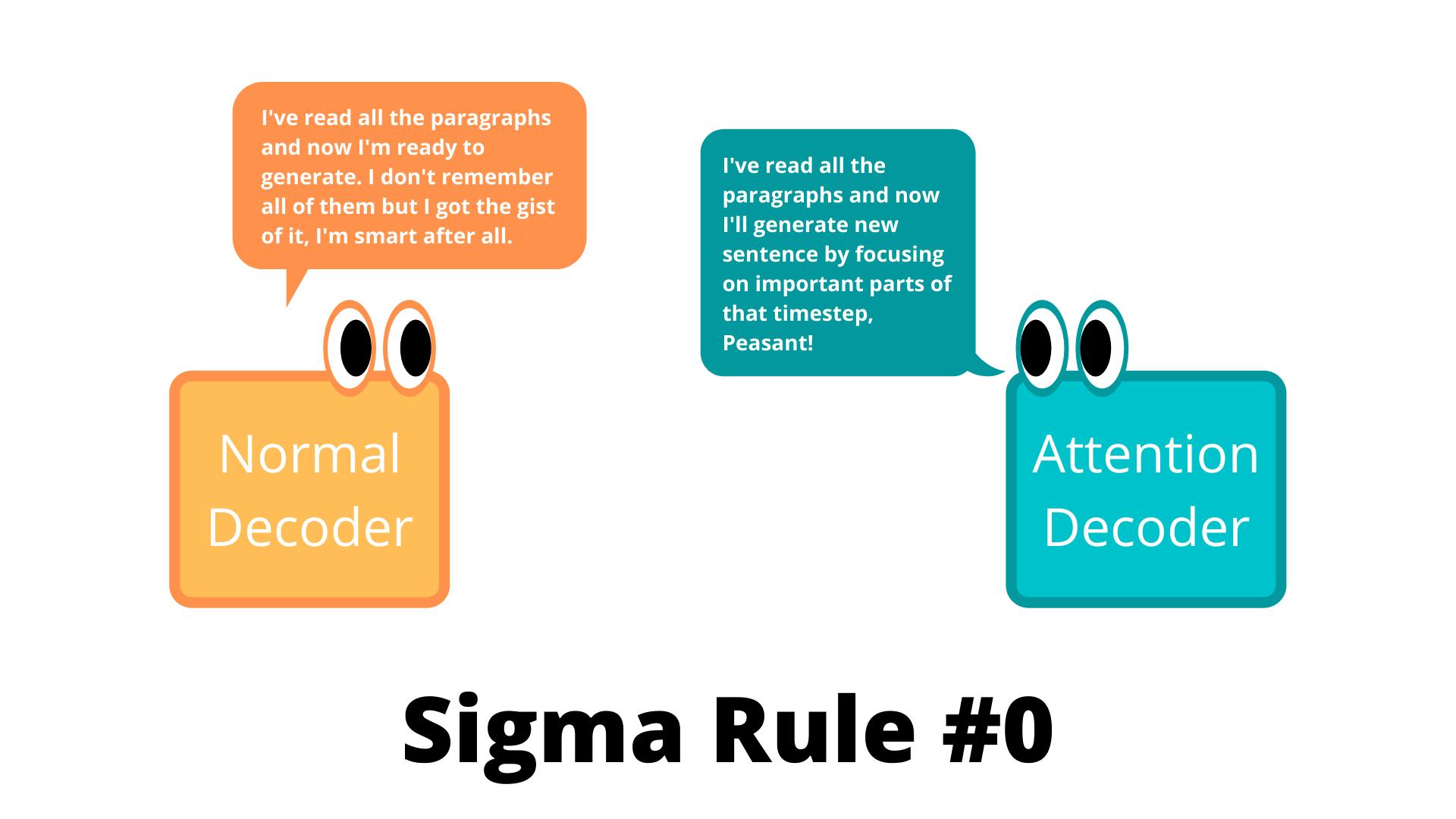
But how does this help? Well, what attention does is that it generates a context vector at each time step of the decoder based on attention score and this attention score helps to amplify the more important words to focus on during that time step in order to improve the quality of results. If you calculate attention among the words of the input sequence it's called Self Attention and when you calculate attention among the words of the input and output sequence it's called General Attention.
Now based on the architecture you have 2 types of attention-based Seq2Seq models i.e. Bahdanau Attention and Luong Attention. Except the architecture and computation both are basically the same but if you wanna learn more you can go ahead and read the paper, Effective Approaches to Attention-based Neural Machine Translation by Luong et. al. 2015.
Scaled Dot-Product Attention
We have a basic idea of how attention works in RNN now, but we don't exactly have an RNN in Transformer or a way to sequentially input data. So the proposed method for calculating attention is via something called Scaled Dot-Product Attention, which is basically a bunch of matrix multiplication operations.
But before diving in, let's talk about QKV or Query-Key-Value vectors and their dimensions. Throughout the model, the dimension of columns of the resultant matrix from each layer is set to 512 which is denoted by \( d_{model} \) .
So if we have m rows in word embedding we'll have the resultant matrix of dimension \( m * d_{model} \) , this column dimension is consistent for all the layers in the model including the embedding layer.
This is done to facilitate the residual connections, which we'll talk about later. Now that we have output dims cleared let's talk about columns of QKV vectors.
For now, just remember the dimension of QKV vectors being 64, the reasoning is something we'll discuss in Multiheaded attention. The dimensions of Query and Key vector are the same and are denoted by \( d_k \) , and even though here it is same the dimensions of value vector can be different and is denoted by \( d_v \) . So to sum it all up we'll have the following notation for dimensions:-
$$d_{model} = 512$$
$$d_q = d_k = 64$$
$$d_v = 64$$
Now that we have the important stuff cleared, let's take a look at the following image that sums up the process of calculating attention:-
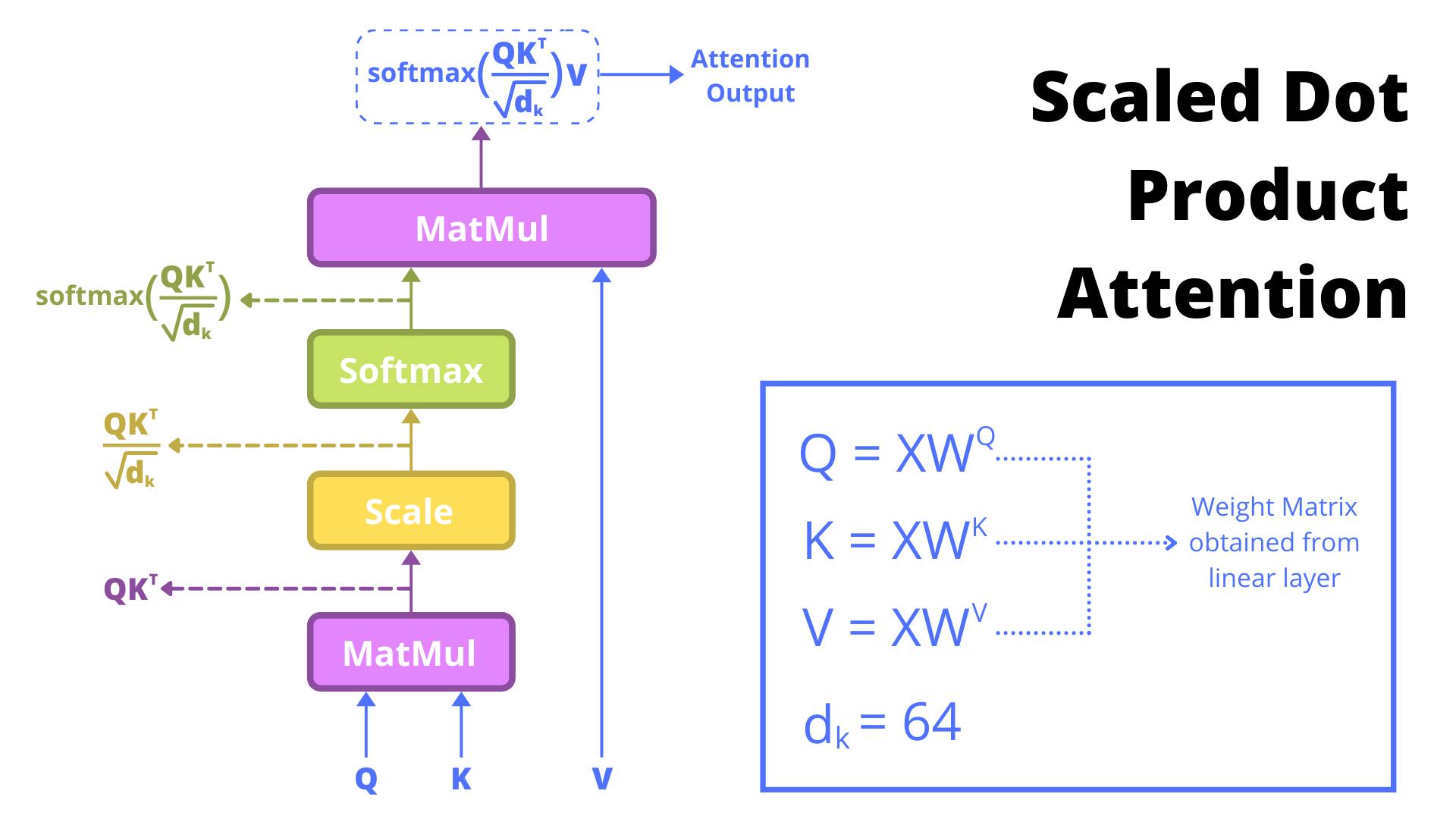
It might seem confusing so let's go in step by step on how attention is being calculated and how its equation is constructed:-
You start by finding Query, Key, and Value vector by multiplying the input matrix with their corresponding weight vector. The dims of these vectors are something we'll discuss in Multi Headed Attention Section. For now, let's just focus on understanding the equation.
\(Attention(Q,K,V)\)
Apply Matrix Multiplication on Query and Key Vector.
\(Attention(Q,K,V)=QKT\)
Scale the result of above with \( \sqrt{d_k} \) . It was observed that for small values of \( d_k \) additive attention and dot product attention perform similarly. But for larger values of \( d_k \) additive attention outperforms dot product attention without scaling. As mentioned in paper, that for large value the result may explode and may push softmax to smaller gradients. To counteract this \( \frac{1}{\sqrt{d_k}} \) was used for scaling. As to why this occurs, paper mentions:-
To illustrate why the dot products get large, assume that the components of q and k are independent random variables with mean 0 and variance 1. Then their dot product has mean 0 and variance d_k.
Applying softmax on the result of the above.
\(Attention(Q,K,V)=softmax((QK^T)/\sqrt{d_k})\)
Apply Matrix Multiplication on result and Value Vector and get the final result.
\(Attention(Q,K,V)=softmax((QK^T)/\sqrt{dk})V\)
There you go that's how you find attention using Scaled Dot Product Attention. Just for the info, this is not the absolute way to find attention, there are other ways to calculate attention like additive attention, dot-product(unscaled) attention. While the two are similar in complexity, dot-product attention is much faster and more space-efficient in practice, since it can be implemented using highly optimized matrix multiplication code.
Now let's take a look at the newly proposed approach where instead of calculating attention one time we calculate it multiple times and then concatenate the results. Yep, it is indeed Multi-Headed Attention.
Multi-Headed Attention
Let's talk about the beast that the paper proposed and when I say "beast" I mean it. The paper suggested that instead of calculating attention one time we can calculate it h times with \(d_q\), \(d_k\), \(d_v\) dimensioned QKV vectors found after passing each of them from a Linear Layer.
We then use them to calculate attention values from each attention head depicted by head_i and concatenate these heads forming \( d_{model} \) dimensional resultant vector. After that, we'll pass them through another linear layer to get our Multi-Headed Attention output. Architecture wise it looks like this:-
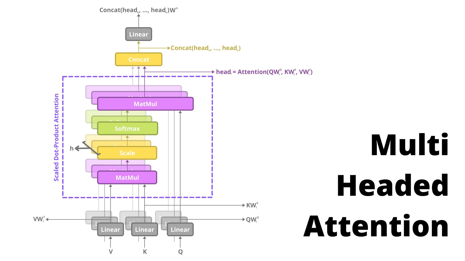
One thing to note is that the value of d_q, d_v, and d_k will be d_model / h, that's why after you concatenate, the attention head's output it becomes d_model sized vector. In this paper, the value of h for the optimal model was 8. So d_k, d_v, and d_q become 512/8 = 64.
Why does it Work?
But after hearing all this it's only sensible to ask. Why does this even work? To answer this query, we should go and take a look at the paper "Analyzing Multi-Head Self-Attention" by Voita et. al. 2019. Where they basically try to find the roles that different attention heads played along with other stuff which we'll talk about later i.e. Attention Head Pruning.
To explain the gist of it the conclusion was, that based on roles attention heads can be divided into 3 parts:-
Positional Heads: Heads where the maximum attention weights was assigned to a specific relative position. This was usually +/- 1 in practice signifying attention to adjacent positions
**Syntactical Heads: ** Head attends to tokens corresponding to any of the major syntactic relations in a sentence. In the paper, they analyze direct relations like nominal subject, direct object, adjectival modifier, and adverbial modifier.
Rare Word Heads: Heads attend to the least frequent tokens in a sentence.
So different heads try to perform different task cool, but do we need all of them? We have only 3 types right? Does that mean other heads are useless? Yes and No. Let's understand the Yes part first.
Yes, attention heads are important and in fact, that's exactly what the blog "Are Sixteen Heads Really Better than One?" by Paul Michael tries to find. In the blog, he tried to explain how the performance was affected when attention heads were pruned. After the experiment they found the following result:-
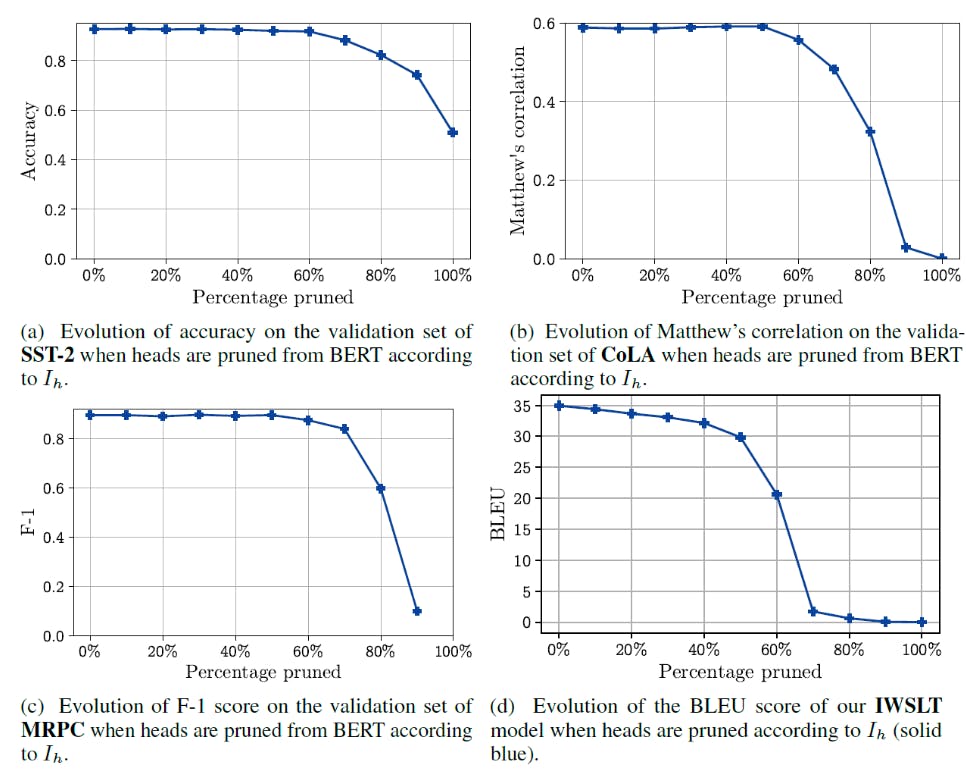
As you can see the BLEU Score is really affected after pruning the heads however like other metrics the dip is observed after more than 60% heads are pruned. This leads us to the No part. I mean kinda No.
Even though we just saw that heads are important we can also prune one or a few of them without seeing a major dip in the performance, something that both the mentioned sources, that I highly recommend you to go through, suggested. Phew that was a lot, now that we have the initial stuff cleared up, let's get back to the architecture. I promise this point forward is a smooth sailing simple life, probably xD.
Encoder
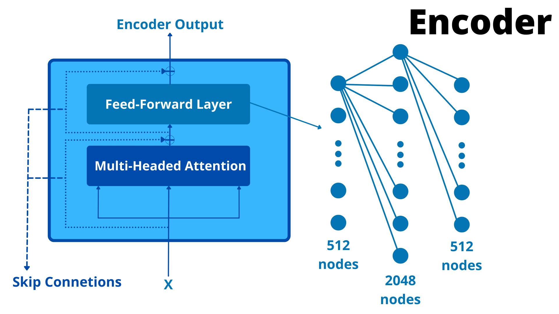
If we try to understand the architecture of Encoder it can be broken into 2 parts:-
Attention Layer
Feed Forward Layer
Yes that's it, you are already familiar with Attention Layer which is nothing but Multi Headed Attention with 8 heads and the Feed Forward Layer is a basic Neural Network with a single hidden layer with 2048 nodes and 512 nodes in input and output layer. Visually it'll look something like this:-
Its flow of Infomation is really simple, or not depending on your knowledge of skip connections. If I have to explain in one line skip connection is basically adding input to the output.
I know it sounds weird, but trust me it makes sense. ResNet model was the one that popularised these skip connections which provides an alternate path for gradients to flow. They helped train deeper models without running into vanishing gradient problem. So if x is the input to a block and f(x) is the output of the block then skip connections basically add them both making x + f(x) the new output.
$$f'(x) = x + f(x)$$
Now that we are all on the same page, let's step by step go through the flow of info in an encoder block:-
Encoder block receives an input X.
X is supplied to Multi-Headed Attention Layer. QKV all will be the same i.e. X.
Multi Headed Attention does the magic and generates an output M(x).
Add X to M(x) because of skip connection.
Apply Layer Normalisation to X + M(x), let's call this N(x).
Pass N(x) to Feed Forward layer to generate an output F(x).
Add N(x) in F(x) because of skip connection again.
Apply Layer Normalisation to F(x) + N(x), let's call this E(x) which is the output of this encoder block.
One last thing, the above is flow of info for one encoder block. This encoder block's output will be passed on to the next encoder block and the architecture of all encoder blocks is the same. The paper proposed the architecture with 6 encoder blocks. I swear I need to learn animation one of these days, would make stuff much much easier.

Yea I know too much info xD, but hey that's all that you need to know about Encoders. The output of the last encoder block is passed to the decoder as KV vector values, which is our next topic of discussion. We are almost near the end, so hang in there 😬.
Decoder
Finally, we are at the last step of the architecture, to be honest decoder is not really that different from than encoder except the fact that here were have an extra layer for masked multi-headed attention. We'll get into the details of that in a bit, but let's get an overview of how a decoder block looks:-
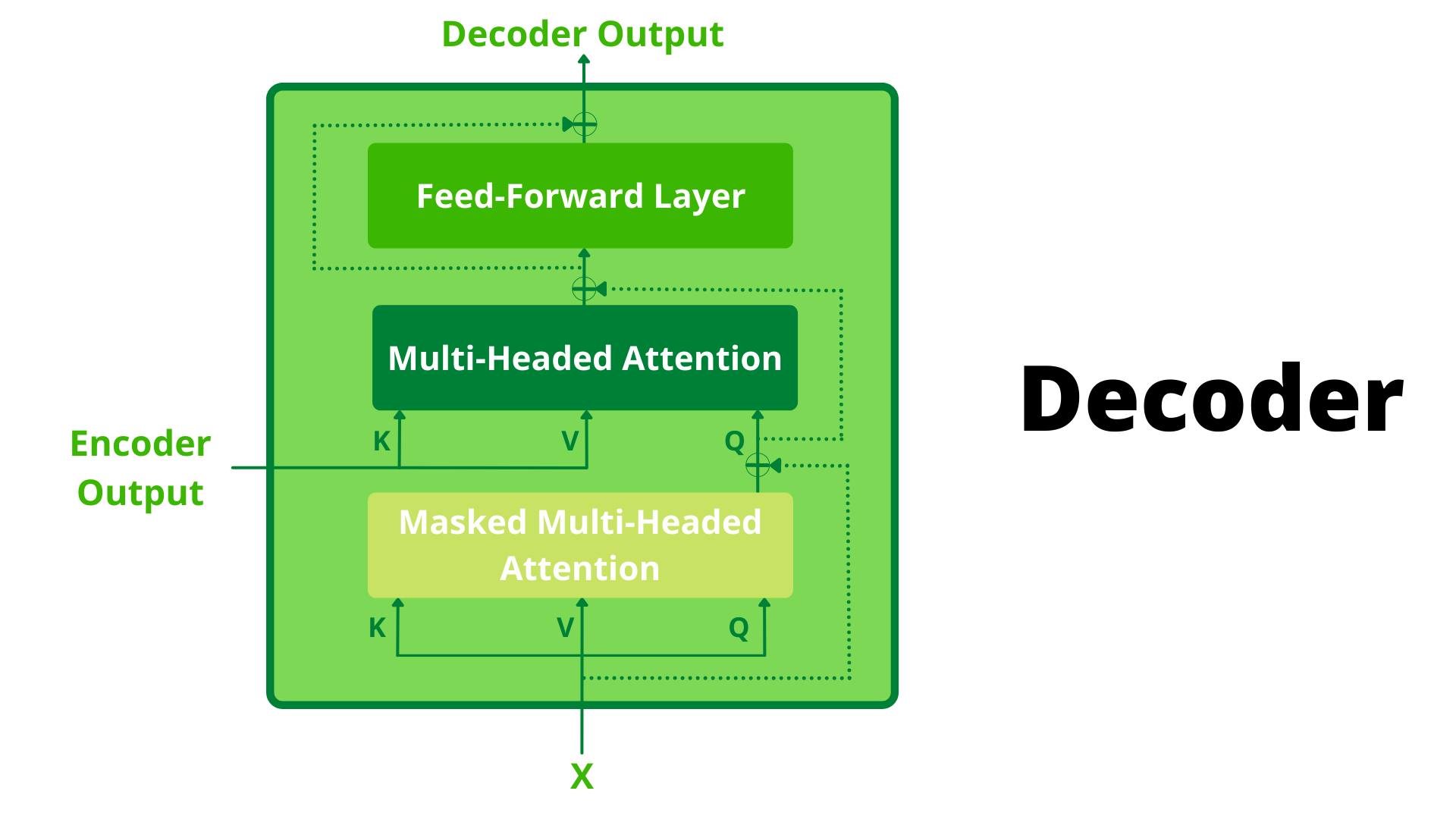
Before going into the flow of information let's understand exactly what is the input and output of the decoder block. As far as input is concerned the decoder takes 2 inputs:-
Encoder Output: This is will be fed as KV Vectors for multi-headed attention in the 2nd layer, this is usually referred to as Encoder-Decoder Attention. All 6 Decoder Blocks will take the encoder output from the last block as input for encoder-decoder attention.
Output Embedding: These are the embeddings of the target sentence. But wait!? We don't have a target in testing! So what are we inputting here then? Let's see.
Well usually the first input to the decoder is a special token signifying the start of the output sentence and the output is the token that comes after this. This output is the output of time step 1.
After that, the input to decoder becomes the tokens until a certain timestep i.e. for the 5th timestep input will be all generated tokens till the 4th timestep. After that, it'll keep on giving an output until it throws a special token signifying the end of the output sentence.
Let's understand the flow of information in decoder block to get a better understanding:-
Decoder block receives an input X.
X is supplied to Masked Multi-Headed Attention as QKV vector, to get an output M(x).
Add X in M(x) because of skip connection.
Apply Layer Normalisation to X + M(x), let's call this N(x).
N(x) is supplied to Multi-Headed Attention as Query and Encoder Output will be supplied as Key-Value..
Multi Headed Attention does the magic and generates an output O(x).
Add N(x) in O(x) because of skip connection.
Apply Layer Normalisation to N(x) + O(x), let's call this P(x).
Pass P(x) to Feed Forward layer to generate an output F(x).
Add P(x) in F(x) because of skip connection again.
Apply Layer Normalisation to P(x) + F(x), let's call this D(x) which is the output of this decoder block.
But all that is nice but how does the decoder predict the next token? Actually, the output of the last decoder block is fed to a Linear Layer that gives an output vector of the size same as that of vocabulary. So depending on how many words the model knows that will be the size of the output vector of this Linear Layer.
Now once you have this vector you apply softmax on this to convert and interpret the values of this vector as probabilities. The token at the index of maximum probability is the output of that "time-step". Take a look at the following infographic to understand it better.
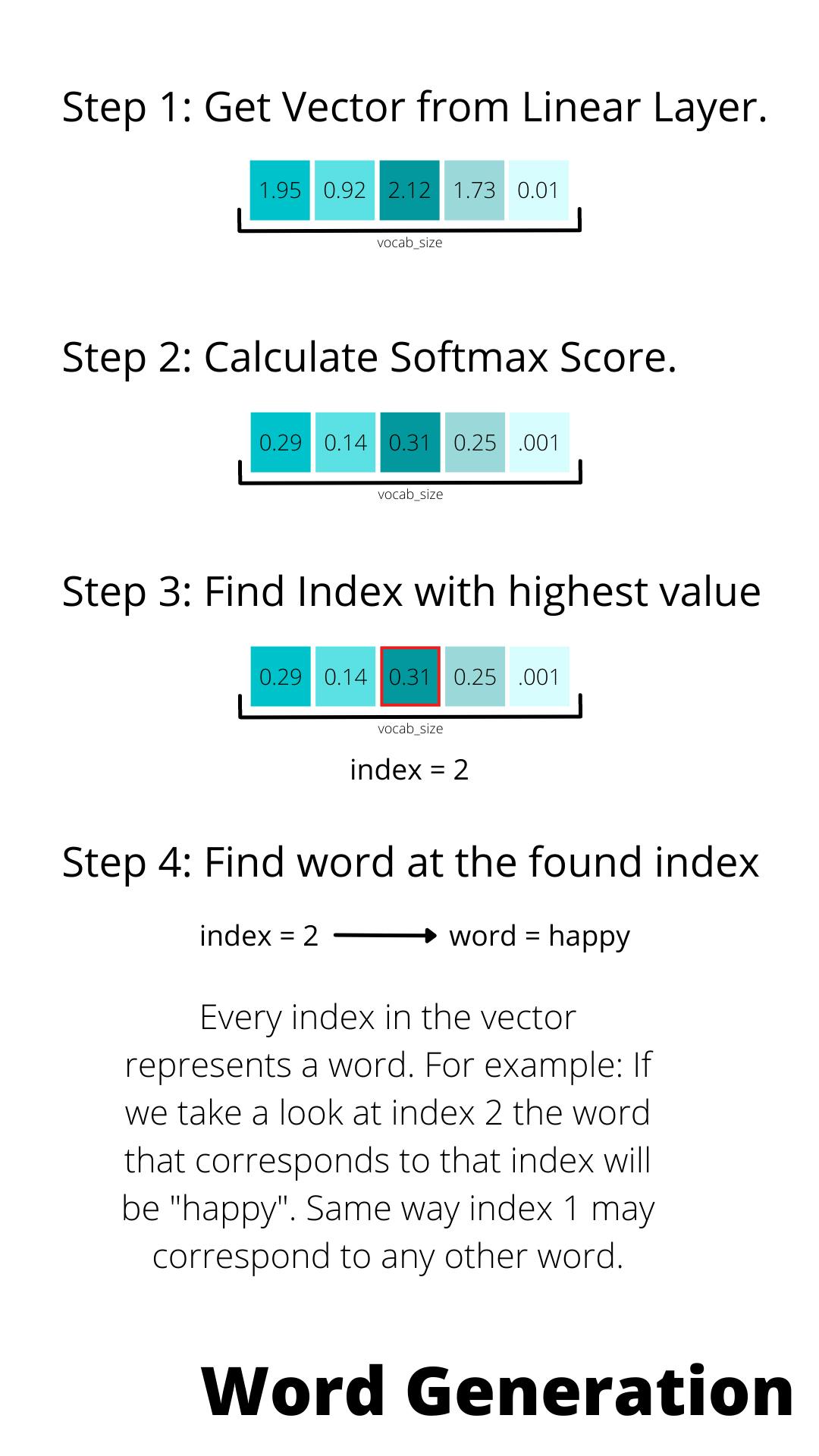
Well, that's basically how the decoder works, but we are still missing one key piece in the puzzle i.e. Masked Multi-Headed Attention. It's actually pretty simple and trust me it won't take much long to understand.
Masked Multi-Headed Attention
If I have to say the difference between Normal Multi-Head Attention and Masked Multi-Head Attention it'll be that in Masked Multi-Head Attention we mask the output of attention score after a point for each token by replacing it with -inf and when it applies softmax these -inf become 0.
Well, that's fine but what exactly is going on? Let's understand. The reason we need such a thing in the first place is so that we can speed up training by being able to compute the probabilities of output token for each input token parallelly. The only reason we are doing this stuff is to speed up training.
And just to be clear this passing all at once stuff is something we'll do only in training, during inference we'll still do it step by step by passing previous outputs to get the new ones.
The aim of an autoregressive model is to find the next step given the previous ones but for parallelization, we'll be passing all the stuff together at once hence we'll need to hide the output of the attention score for the future time steps of that token to properly train the model. Let's understand this step by step to get a better understanding.
Step-By-Step Guide to Masked MHA
So let's start by knowing what exactly we need to find:-
$$P(x_{i+1}|[x_0, x_1, ..., x_i])$$
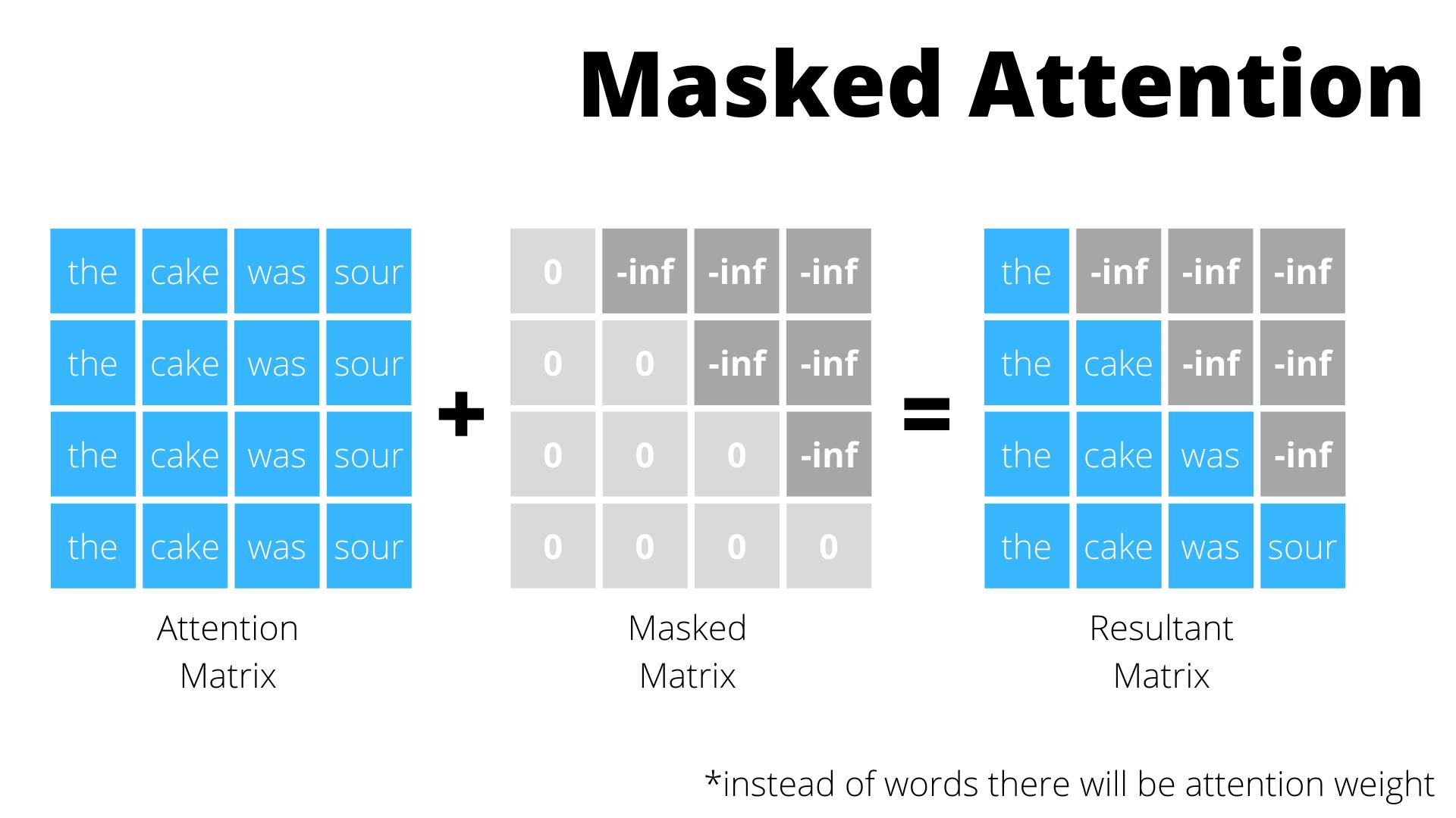
What the above equation means is that we'll need to find the probability of the next word given the previous ones in sequence. Now let's consider the following sentence and let's assume it to be the expected output:-
$$The \space cake \space was \space sour$$
If you pass words one by one you prevent seeing the future steps but for efficiency, you'll need to pass all the words together. When you do this you expose the decoder to future info, in order to prevent that we mask the weights of all j(>i) future steps, i being the current time step.
So for the word cake in the above sentence, we'll mask the weight for words was and sour, the same way for the word was in the above sentence we'll mask the weight for sour. We can do this by adding a mask matrix to this:-
Implementation-wise, you apply the mask after doing the scaled matrix multiplication of the QV vector in scaled dot product attention. After this you proceed normally, the only difference is this masking step.
Training and Results

Done! We are done with the architecture. We are officially out of the deadly stuff and now it's just simple stuff. So let's wrap it up. Let's start by going through some details regarding the training:-
Data: The WMT English German Dataset contained 4.7 million sentence pairs, with a vocabulary of about 37k tokens. The WMT English French Dataset contained 36 million sentence pairs, which is so big that my hard drive will die before loading it.
Hardware: Richie Rich people xD. Trained on 8 Nvidia P100 GPU something which make me go bankrupt 100 times. Trained for 100k steps for 12hrs. The bigger variants were trained for 300k steps for 3.5 days.
Optimizer: They used Adam optimizer with β1 = 0.9, β2 = 0.98 and epsilon = 10^−9. Increasing the learning rate linearly for the first warmup_steps training steps, and decreasing it thereafter proportionally to the inverse square root of the step number. They used warmup_steps = 4000.
**Regularization: ** Dropout of 0.1 was applied to the sum of the positional and wor embeddings. Dropout was also applied to the output of the sublayer before the residual step. Label smoothing was also applied with epsilon = 0.1. Label Smoothing is a way to prevent the model from being too confident about it's prediction.
That's all as far as training is concerned. Now the architecture I explained had very specific parameters but that's not the only model they tried. They actually tried a bunch of them and noted the result of each in the table below:-
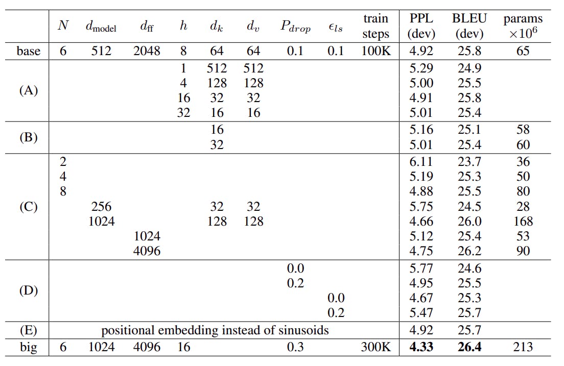
As you can see big model performed the best out of all but between big model and base model with a small performance drop, I'll take my chance with the base one first.
That's all! We have finished the paper and reached the end, take a moment and clap for yourself.

From Me to You...
Wow, that was a big blog and I won't lie it was tough to write. This is probably one of my longest and most experimental blog ever. I was super casual and explained everything as much as possible. At some point I wanted to just stop but every time I just thought, just a bit more.
Transformers are probably one of those revolutionary concepts in deep learning that changed the way we approached stuff and I hope I was able to dissect the paper that started it all. I hope you had fun reading it.
Forever and Always, Herumb.